Getting Started

Every time I start a new machine learning project (not deep learning, that’s a story for another time), I find myself going through the same tedious process of trial and error - set up a grid search to find the right model along with the right set of hyperparameters for the model that optimize one or more of the laundry list of metrics-of-interest…then repeat every combination of free parameters in this pipeline a bunch of times and finally making a lot of plots to get the lay of the land so to speak. So, over the years, I’ve developed a set of convenience wrappers around the mighty scikit-learn library to make this process a bit more streamlined and I’ve published them as clfutils4r for classification tasks and clustutils4r for clustering tasks (the ‘r’ being my initial and not the programming language…err, should have thought this through, huh?). I thought I would share them here in case they are useful to anyone else.

Classification

The premise is this: Someone hands you a classification dataset. After you are done poking and prodding it with some exploratory data analysis (EDA), you want to know the standard metrics on various classifiers available in scikit-learn and you want to know them now. You don’t want to spend time writing boilerplate code setting up a grid search and you don’t want to spend time making plots to consolidate the results of said grid search. Here is minimally complete example of how you can do just that with 2 wrapper functions:

import matplotlib.pyplot as plt
import numpy as np
import pandas as pd
import os

from sklearn import datasets
from sklearn.preprocessing import StandardScaler

## Load dataset: Example - breast cancer prediction
data = datasets.load_breast_cancer()
class_names = [str(x) for x in data.target_names]
feature_names = [str(x) for x in data.feature_names]
X, y = data.data, data.target

## Standardize features
scaler = StandardScaler()
X = scaler.fit_transform(X)

## Split into train and test sets
from sklearn.model_selection import train_test_split
X_train, X_test, y_train, y_test = train_test_split(X, y, test_size=0.30, random_state=42)

## Grid search for best model
from clfutils4r.gridsearch_classification import gridsearch_classification
save_dir = "gridsearch_results"
os.makedirs(save_dir, exist_ok=True)
best_model, grid_search_results = gridsearch_classification(X=X_train,                    # training dataset
                                                            gt_labels=y_train,            # ground truth labels
                                                            best_model_metric="F1",       # metric to use to choose the best model
                                                            show=True,                    # whether to display the plots; this is used in a notebook
                                                            save=True, save_dir=save_dir  # whether to save the plots
                                                        )

## Predict on test set
y_pred = best_model.predict(X_test)
y_pred_proba = best_model.predict_proba(X_test)

## Evaluate best model on test set
from clfutils4r.eval_classification import eval_classification
eval_classification(y_test=y_test, y_pred=y_pred, y_pred_proba=y_pred_proba,  # ground truth labels, predicted labels, predicted probabilities
                    class_names=class_names, feature_names=feature_names,
                    make_metrics_plots=True, # make a variety of classification metrics plots
                    make_shap_plot=True, shap_nsamples=100, # do Shapley analysis for model explainability
                    show=True,  
                    save=True, RESULTS_DIR=os.getcwd()+'/test_results')

Let’s dive a bit deeper into these two convenience functions.

gridsearch_classification

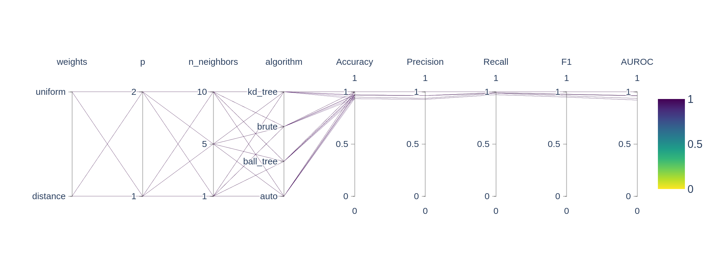
This will produce a whole bunch of useful outputs including the best model and the results of the grid search. The data is stored in neat folder structure in JSON files and is visualized with a Parallel Co-ordinates Plot.

eval_classification

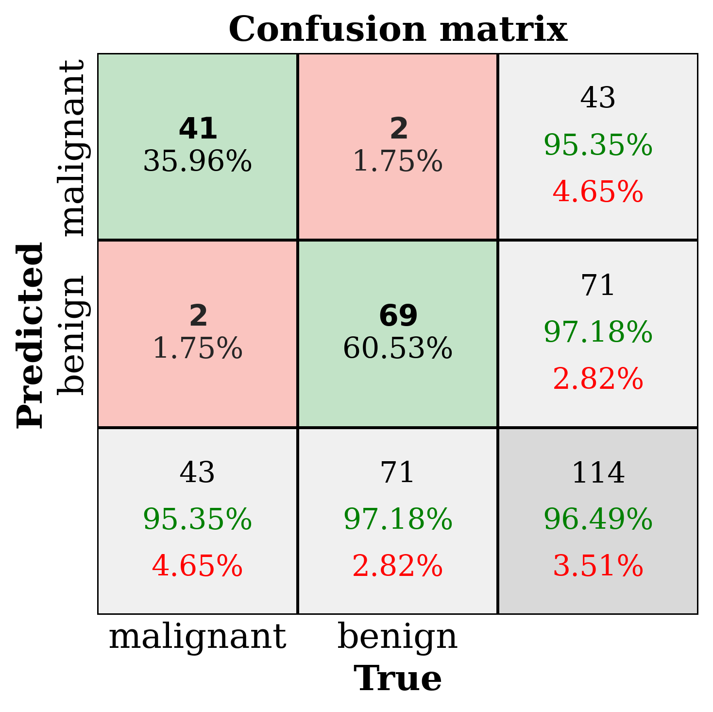
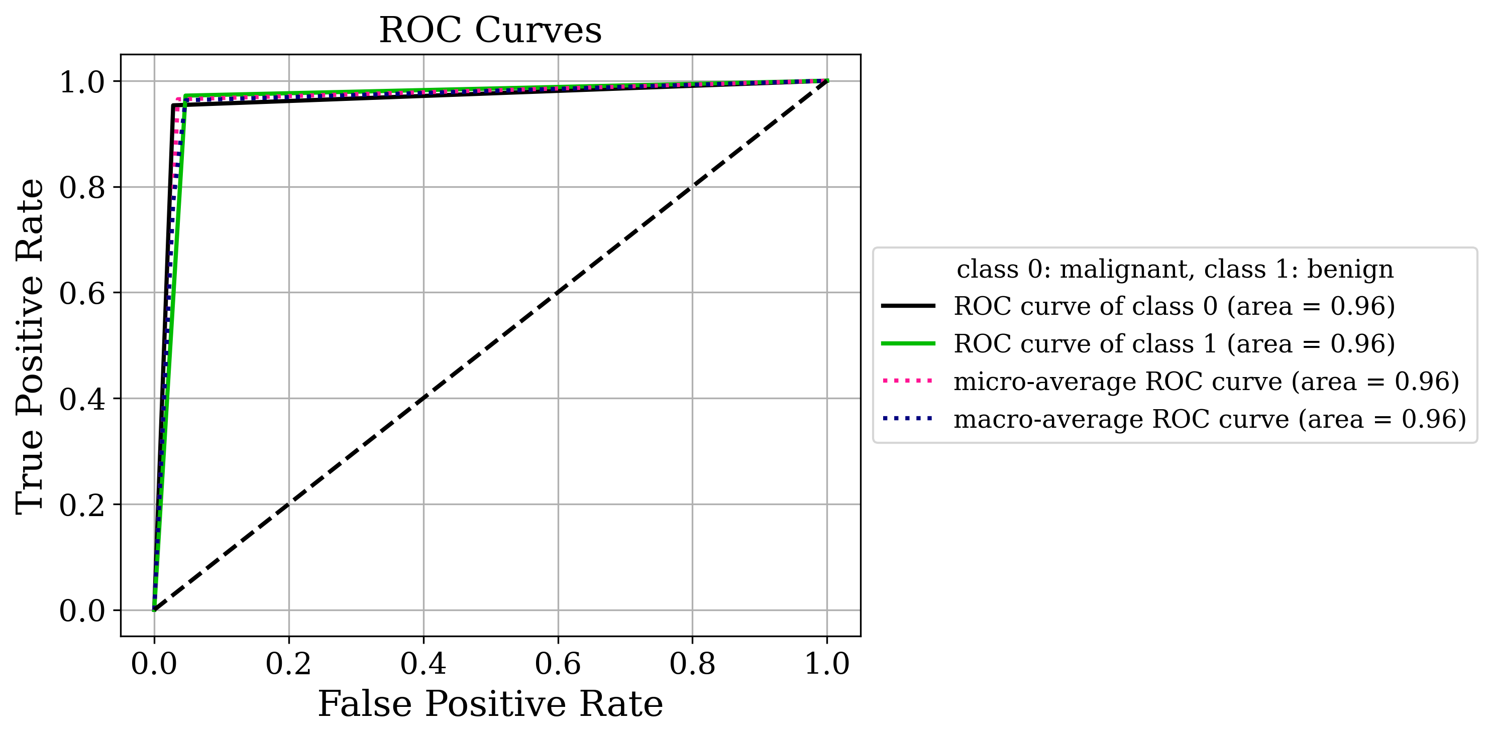
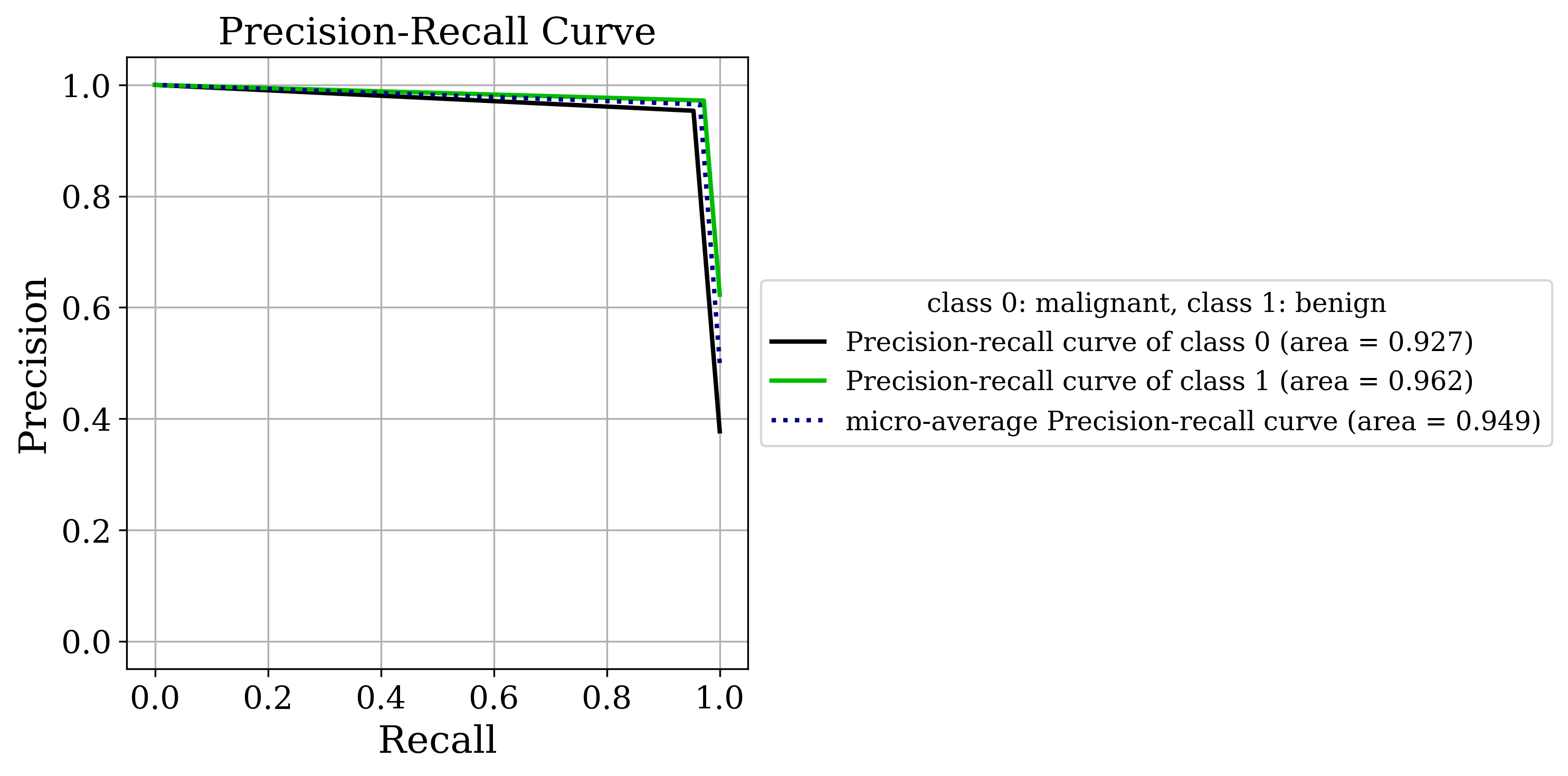
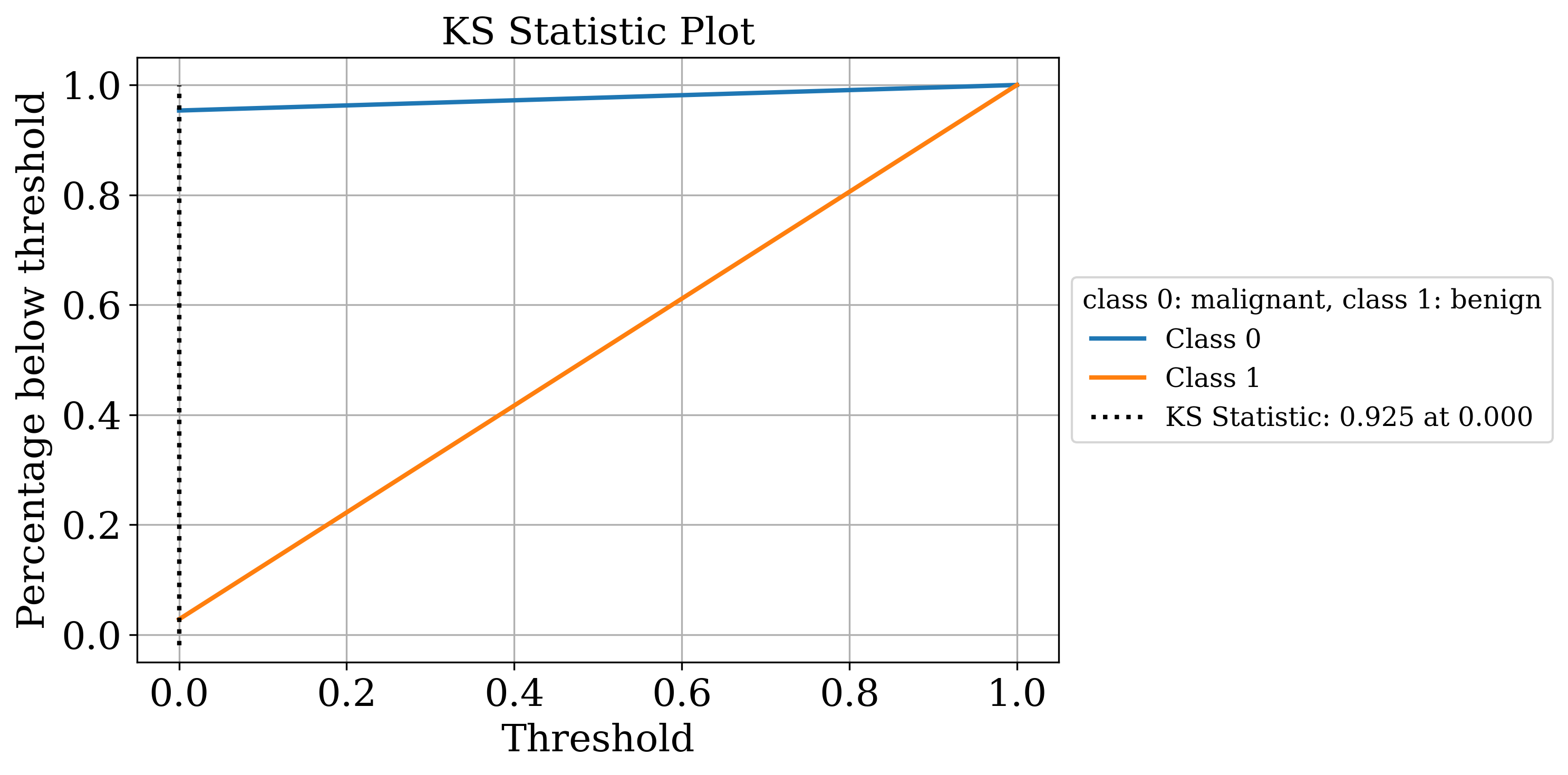
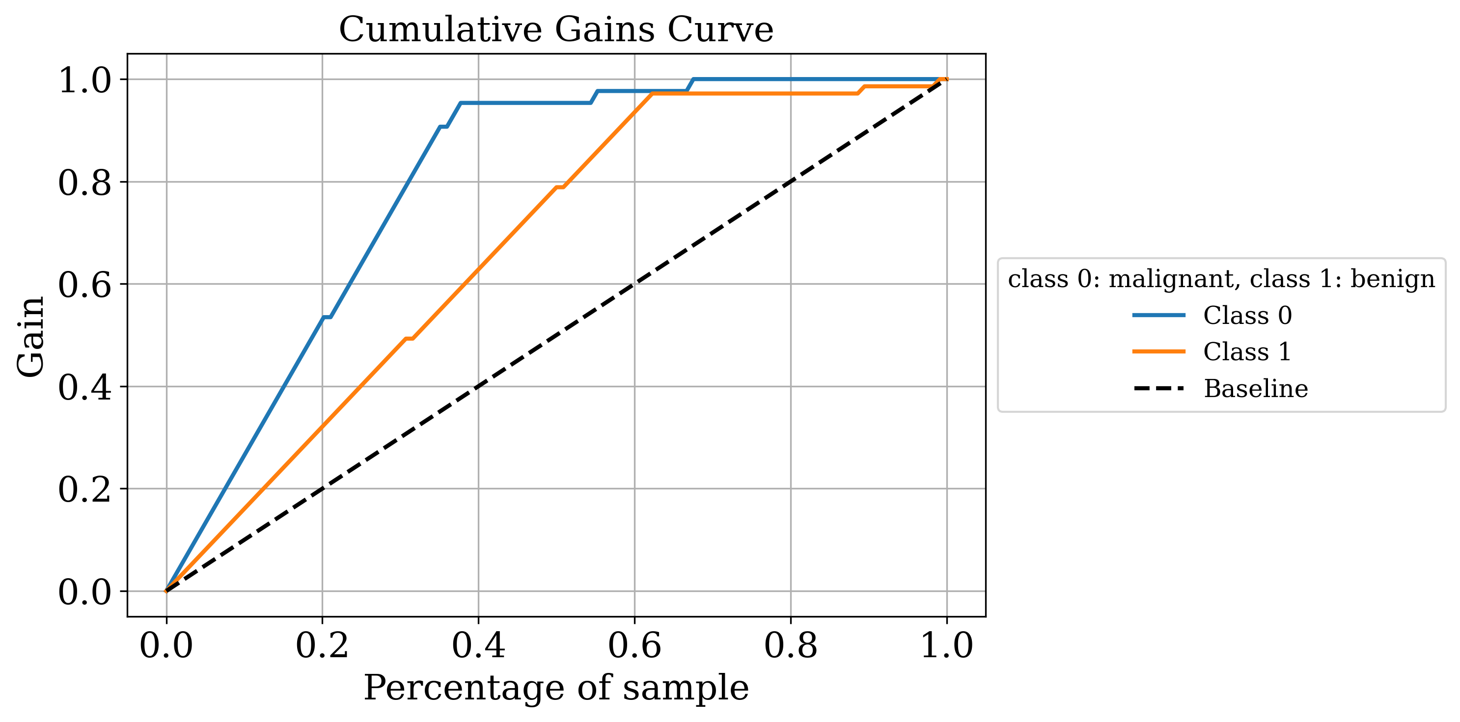
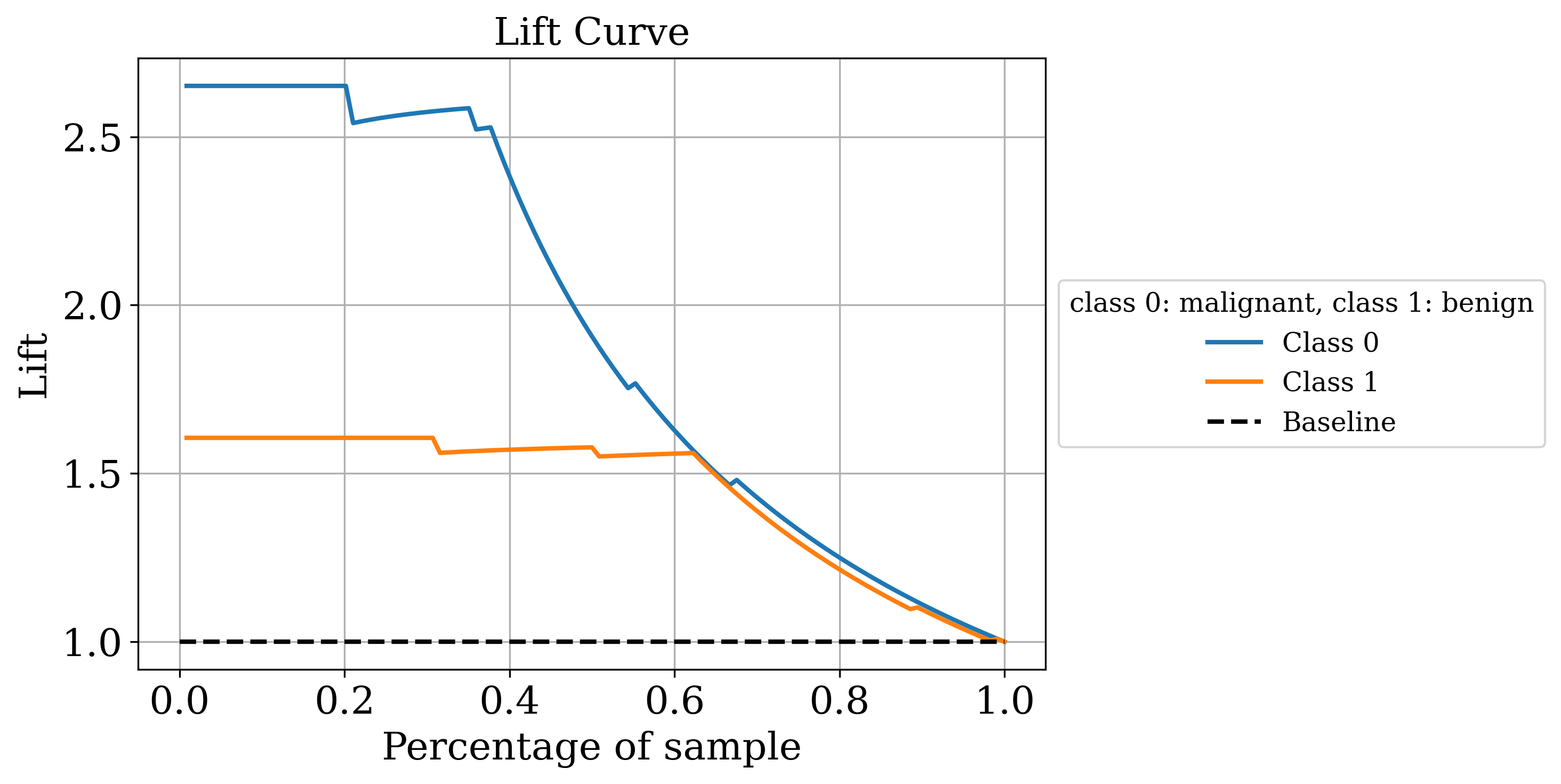
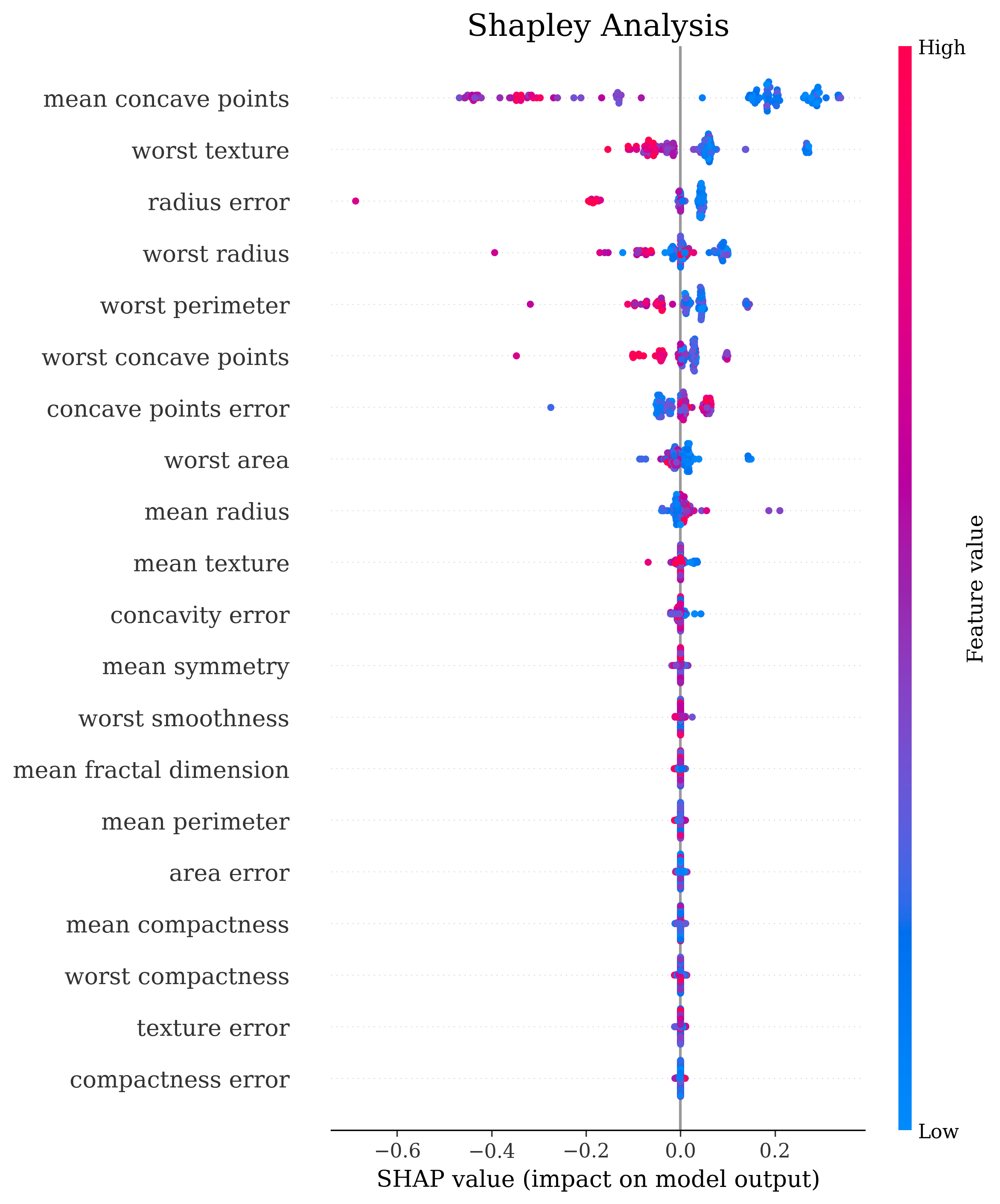
The primary output is the classic sklearn classification report. Sometimes that’s all you need but by setting the make_metrics_plots to True you can choose to make a variety of other plots that I find useful for understanding the performance of the model. These include the familiar plots of the confusion matrix, the ROC curve, the precision-recall curve as well as some more exotic ones I found in scikit-plot that are exclusive to binary classification like the KS statistic plot, the cumulative gains curve and the lift curve. You can also choose to do Shapley analysis to explain the model predictions by setting the make_shap_plot parameter to True and specifying the number of samples to use for the analysis with the shap_nsamples parameter. I love the fantastic shap package so I just wrapped the KernelExplainer and summary_plot in this function.

Clustering

Same premise as before but this time with clustering tasks. Here is a minimally complete example of how you can do it with 1 function:

import os
import numpy as np
from sklearn.datasets import make_blobs
from clustutils4r.eval_clustering import eval_clustering

## For testing purposes
rng = np.random.RandomState(0)
n_samples=1000

### Synthetic data
X, y = make_blobs(n_samples=n_samples, centers=5, n_features=2, cluster_std=0.60, random_state=rng)

save_dir = "results"
os.makedirs(save_dir, exist_ok=True)

best_model, grid_search_results = eval_clustering(
                                       X=X,                                               # dataset to cluster
                                       gt_labels=y,                                       # ground-truth labels; often these aren't available so don't pass this argument
                                       num_runs=10,                                       # number of times to fit a model
                                       best_model_metric="Calinski-Harabasz",             # metric to use to choose the best model
                                       make_silhoutte_plots=True, embed_data_in_2d=False, # whether to make silhouette plots
                                       show=True,                                         # whether to display the plots; this is used in a notebook
                                       save=True, save_dir="results"                      # whether to save the plots
                                    )

Clustering, as you know, is a bit trickier than classification because often there is no ground truth to compare the found clusters to. There is also rarely some external validation test or downstream task available to quantify if any/all clusters you found are “useful”. Clustering is often an exploratory tool. So, the evaluation is a bit more heuristic based. Clustering also often has one or more free parameters, for example, the number of clusters in case of partition-based algorithms like K-Means or the minimum cluster size in case of density based algorithms. In sklearn there are 3 intrinsic cluster quality metrics viz. the Calinski-Harabasz score, the Davies-Bouldin score and the most used one being the Silhouette Score. Another important evaluation folks do for clustering is measuring the consensus between different labellings of the same dataset. sklearn has a wide variety of clustering consensus metrics like Adjusted Rand Index, Normalized Mutual Information, V Measure, Fowlkes-Mallows Index.

Let’s take a look at my convenience function.

eval_clustering

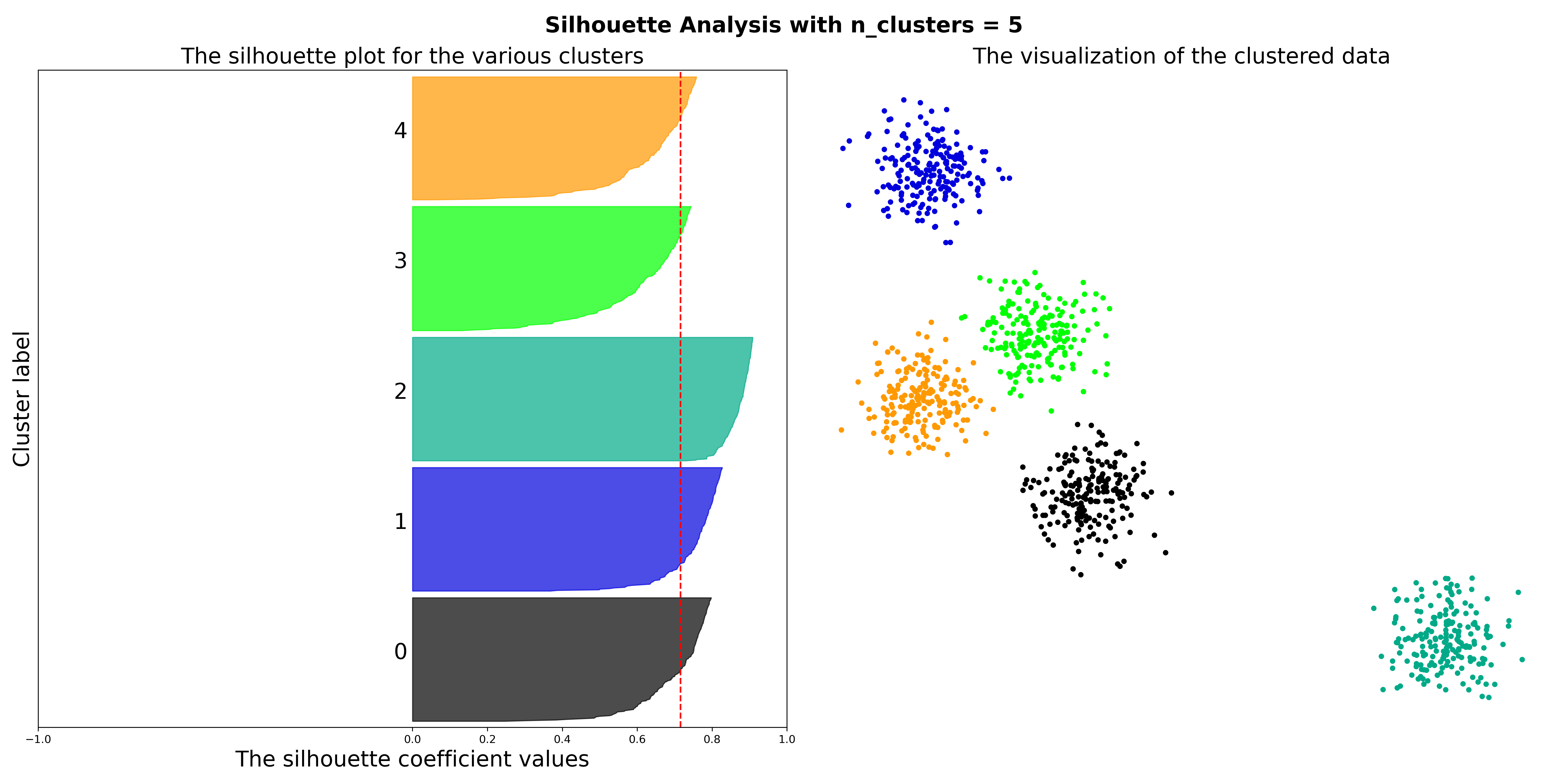
In the default setting in which all you have is the unlabelled dataset, it will calculate the three intrinsic cluster quality metrics for a variety of models and combinations of free parameters and return the best model based on the scoring metric you choose using the best_model_metric parameter along with the full grid search results. You can also make a Silhouette Plot for the best model by setting the make_silhoutte_plots to True and since most datasets have more than 2 features, you can get a t-SNE projection of the high dimensional datapoints by setting embed_data_in_2d to True. If you have the ground truth labels (or just another set of labels obtained by, say, a different clustering run) available, you can pass them to the gt_labels parameter and it will calculate the clustering consensus metrics.

Parting Thoughts

Every machine learning engineer, researcher and dabbler I’ve met over the years has their own version of such wrappers. I hope someone finds these ones useful. I’ve packaged and published these on PyPI; install them with pip install clfutils4r and pip install clustutils4r. The code is available on my Github, fork away and modify to your liking. Even if you don’t like them as they are, hopefully they save you some time by serving as a starting point. Recently, I’ve taken to using Optuna for hyperparameter optimization and I’m thinking of incorporating that into these wrappers. It has a lot cleverer ways of optimally searching the hyperparameters space than the good old GridSearchCV and RandomizedSearchCV that I’ve been using here. I would like to point to PyCaret which is a fantastic low-code, scikit-learn wrapper library that does a lot of what I’ve done here and so much more; it has a truly eye-watering amount of options one can play with and it integrates pretty much every hyperparameter search package available including Optuna, Ray Tune, Hyperopt, Scikit Optimize (which is probably defunct now?). PyCaret has everything one would need for classification, especially the compare_models() function which is fantastic for getting a quick models x metrics table comparing all available models via cross-validation and tune_model() which essentially does what my gridsearch_classification() does and returns the best model and optionally the tuner object from which you can grab the full grid of results. As of this post, I haven’t seen similar functions in the clustering module of PyCaret but I’m sure they are on the way. I’ve used it a few times and it’s great but I wanted to write my own wrappers to understand the process better. Thanks for reading this post!